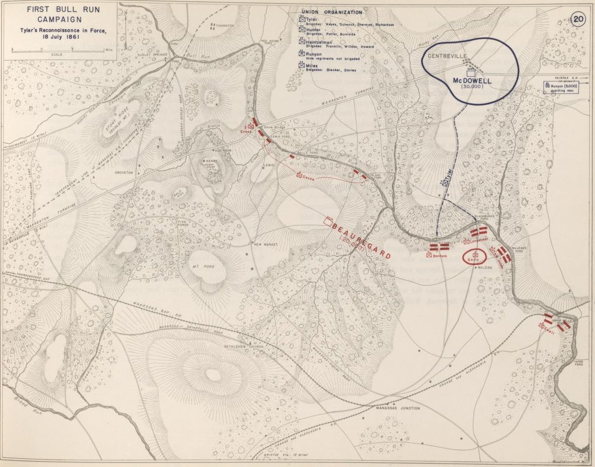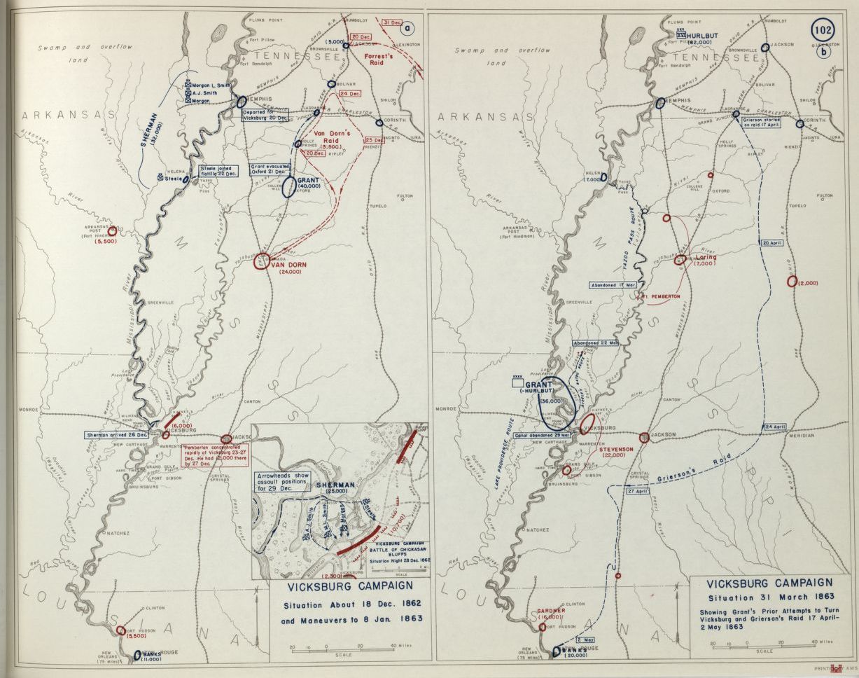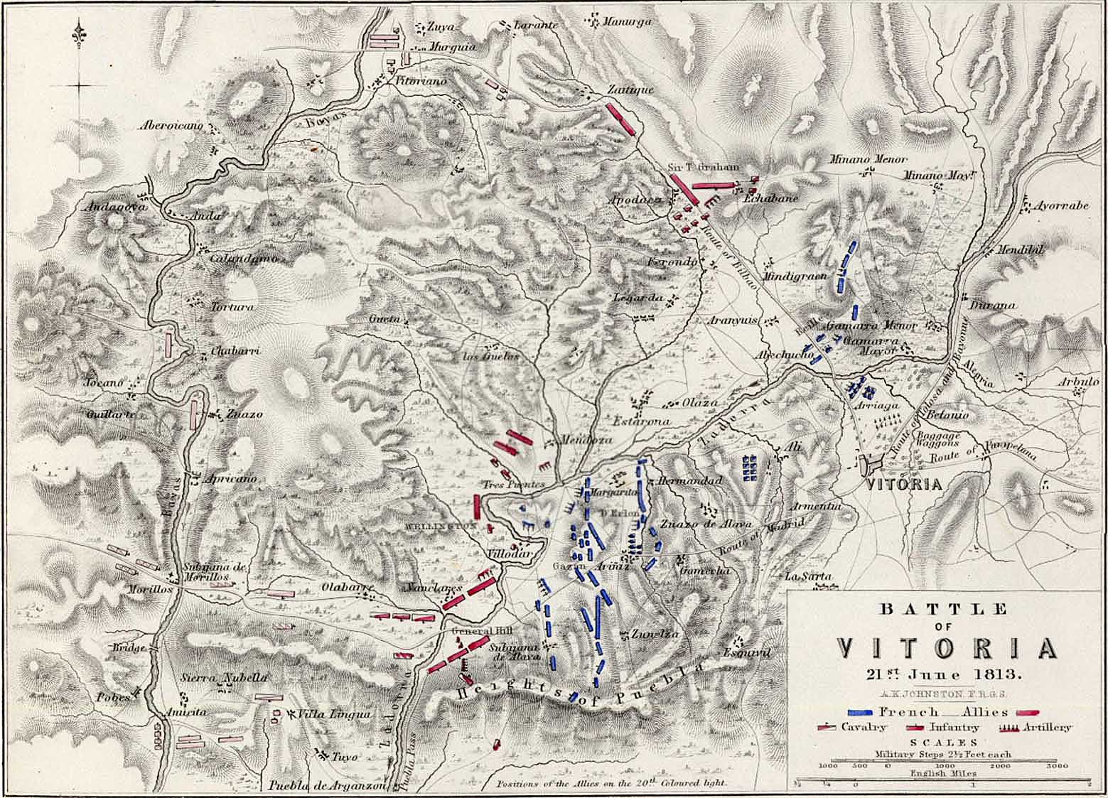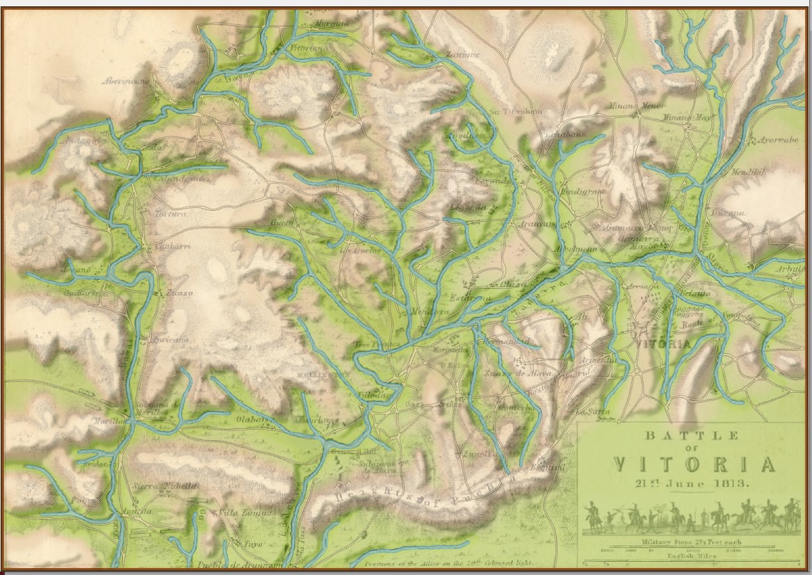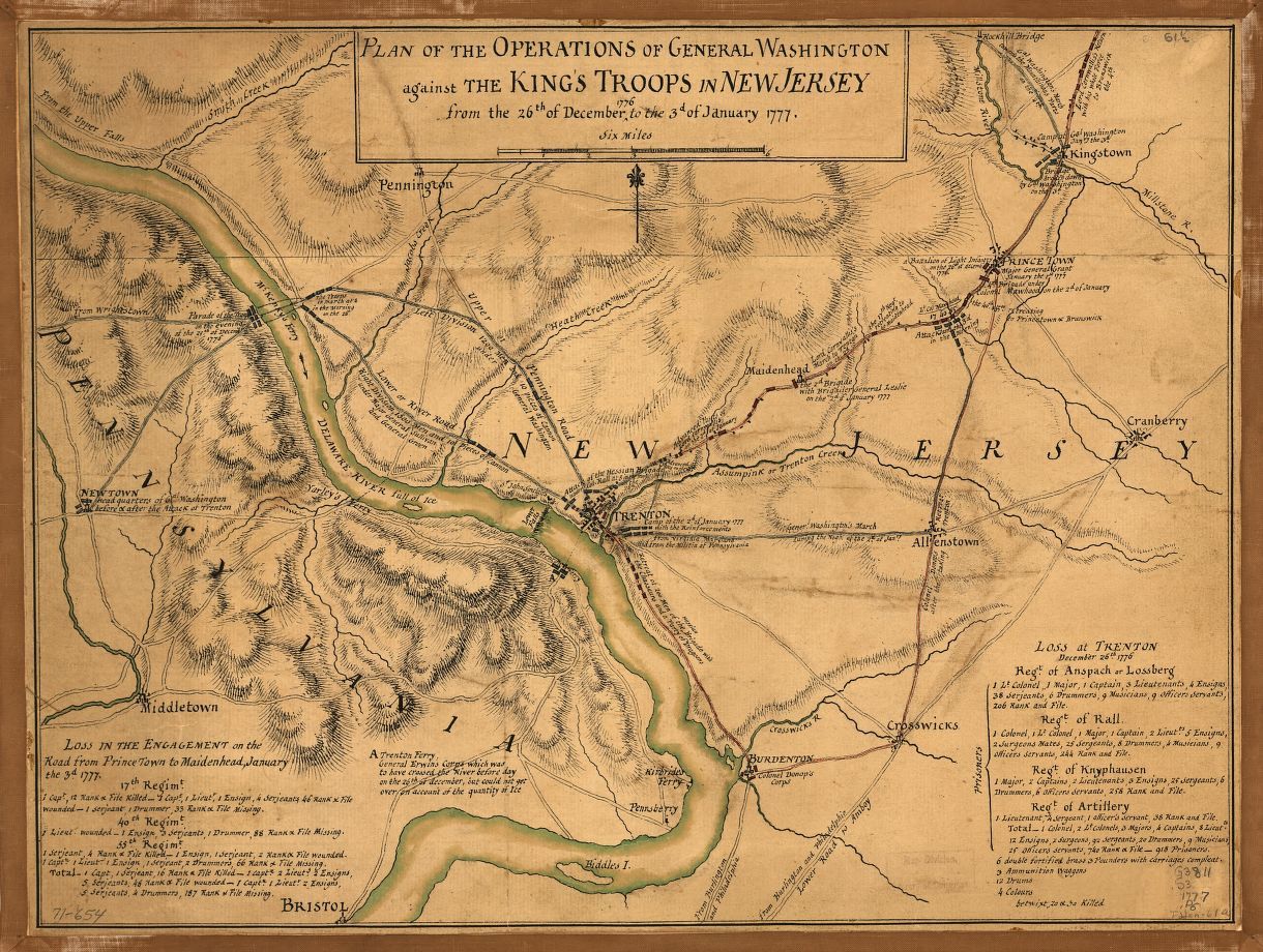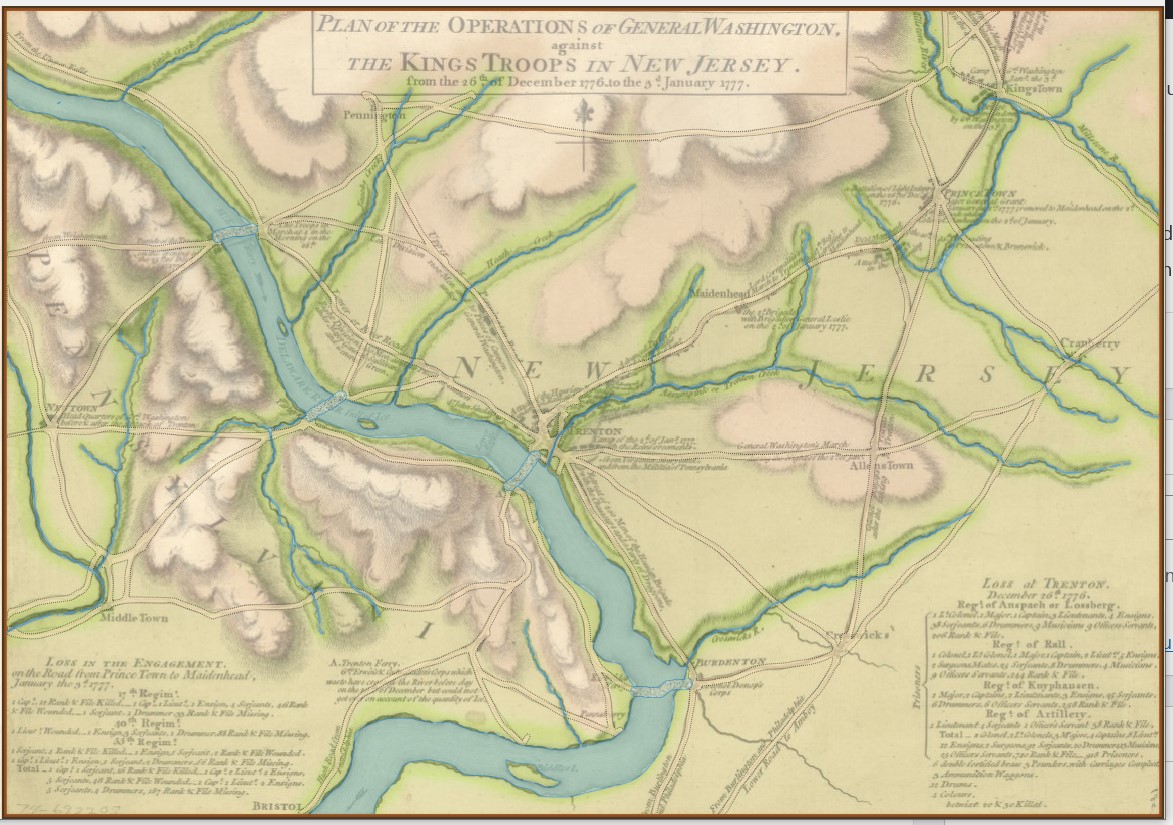
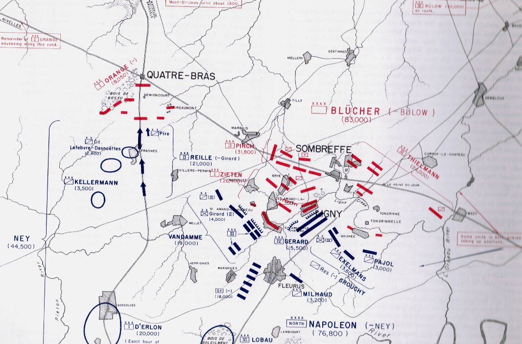
Map 159 from the superb, “West Point Atlas of the Napoleonic Wars,” (Esposito & Elting, 1999, Stackpole). Scanned from the author’s collection. Click to enlarge.
The seeds of Napoleon’s defeat at Waterloo were sown two days earlier at his victory near Ligny. Napoleon needed to surround and completely remove the Prussian army as a viable force on the battlefield. Instead, they escaped to Wavre in the north and resurfaced at the worst possible time on Napoleon’s right flank two days later at Waterloo.
MATE1)Machine Analysis of Tactical Environments 2.0 is now capable of analyzing the battle of Ligny, June 16, 1815 from both the Blue (L’Armée du Nord on the offensive) and Red (Prussian on the defensive) positions. (MATE is the AI behind General Staff: Black Powder. For more information about MATE see these links).
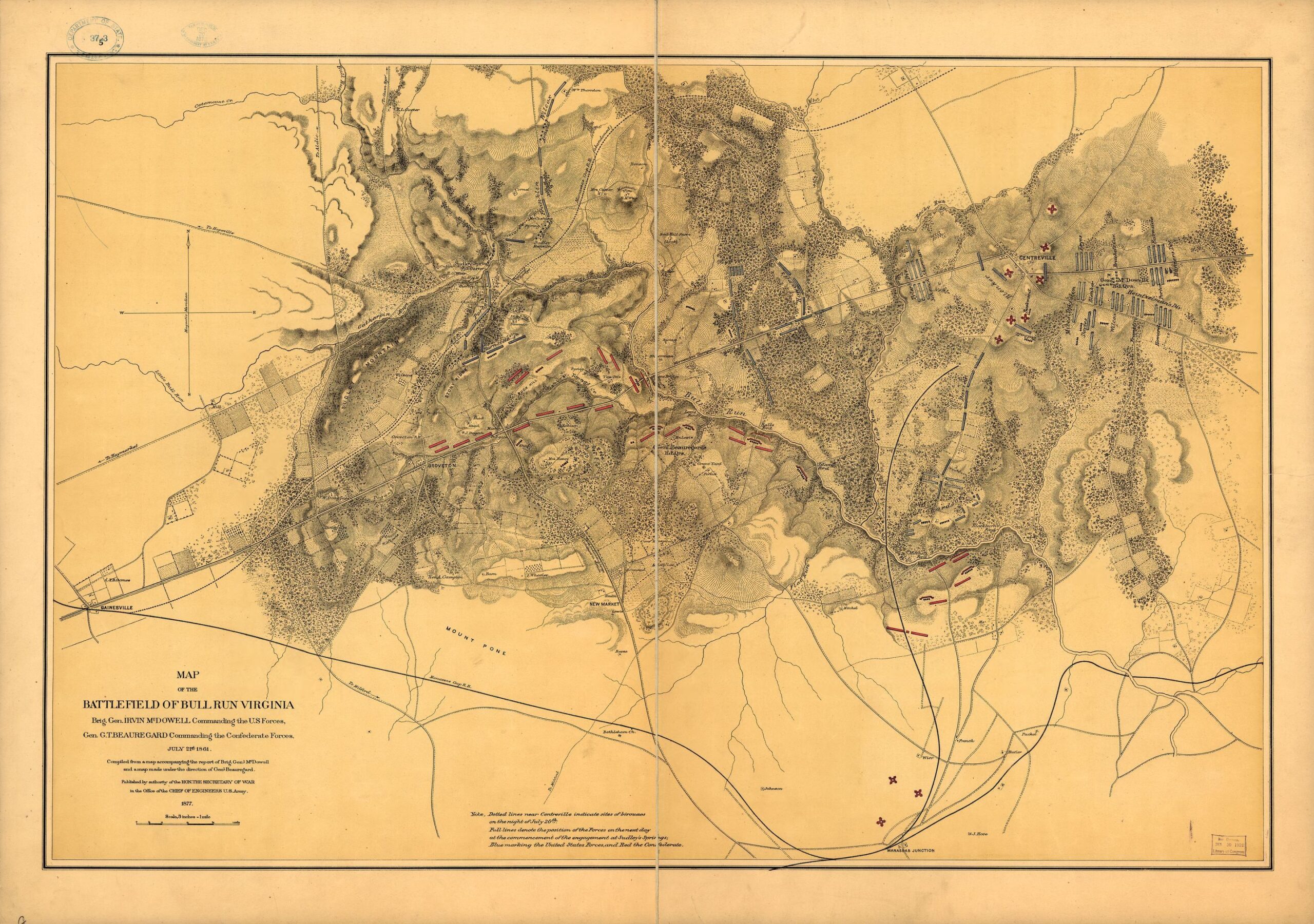
The Ligny map was donated by Glenn Frank Drover. Jared Blando is the artist. Ed Kuhrt did the elevation, roads and mud terrain overlays. The unit positions are from the West Point Atlas of the Napoleonic Wars (above) and from David Chandler’s Waterloo: The Hundred Days. If any one has a better source for unit positions, please contact me directly.
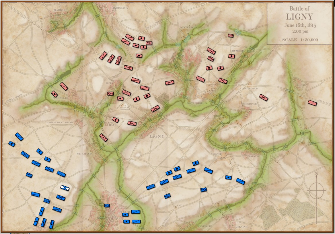
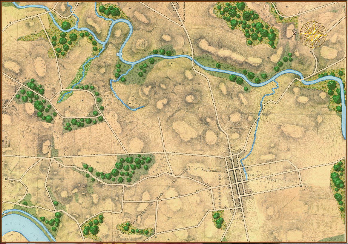
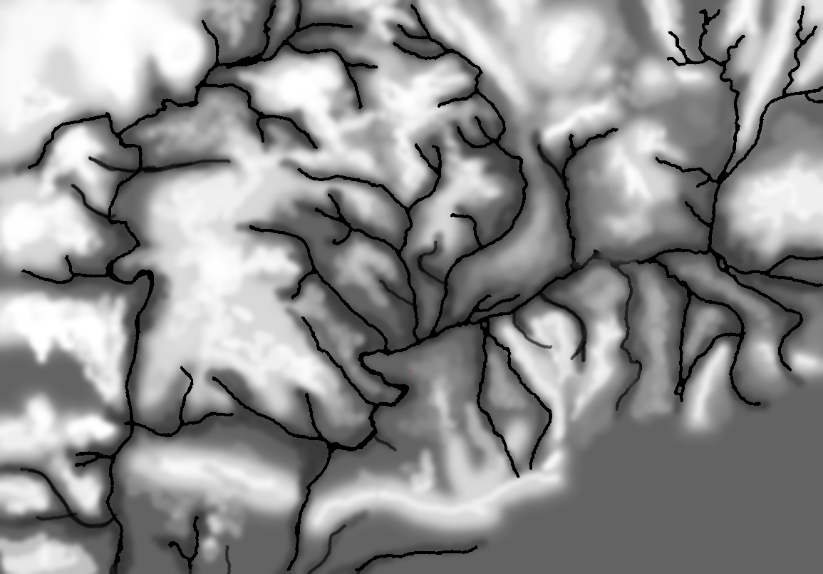
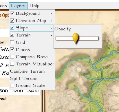
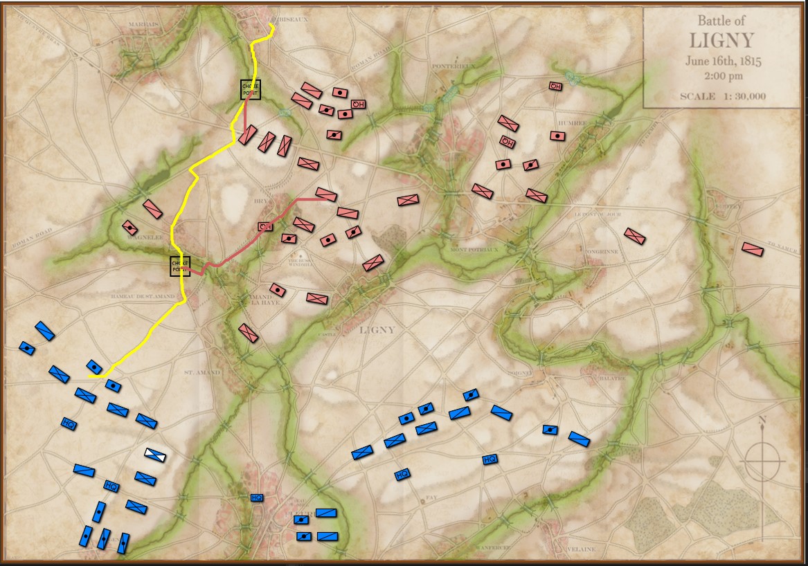
Screen capture of the Ligny scenario in General Staff. Elevation and slope layers enhanced.
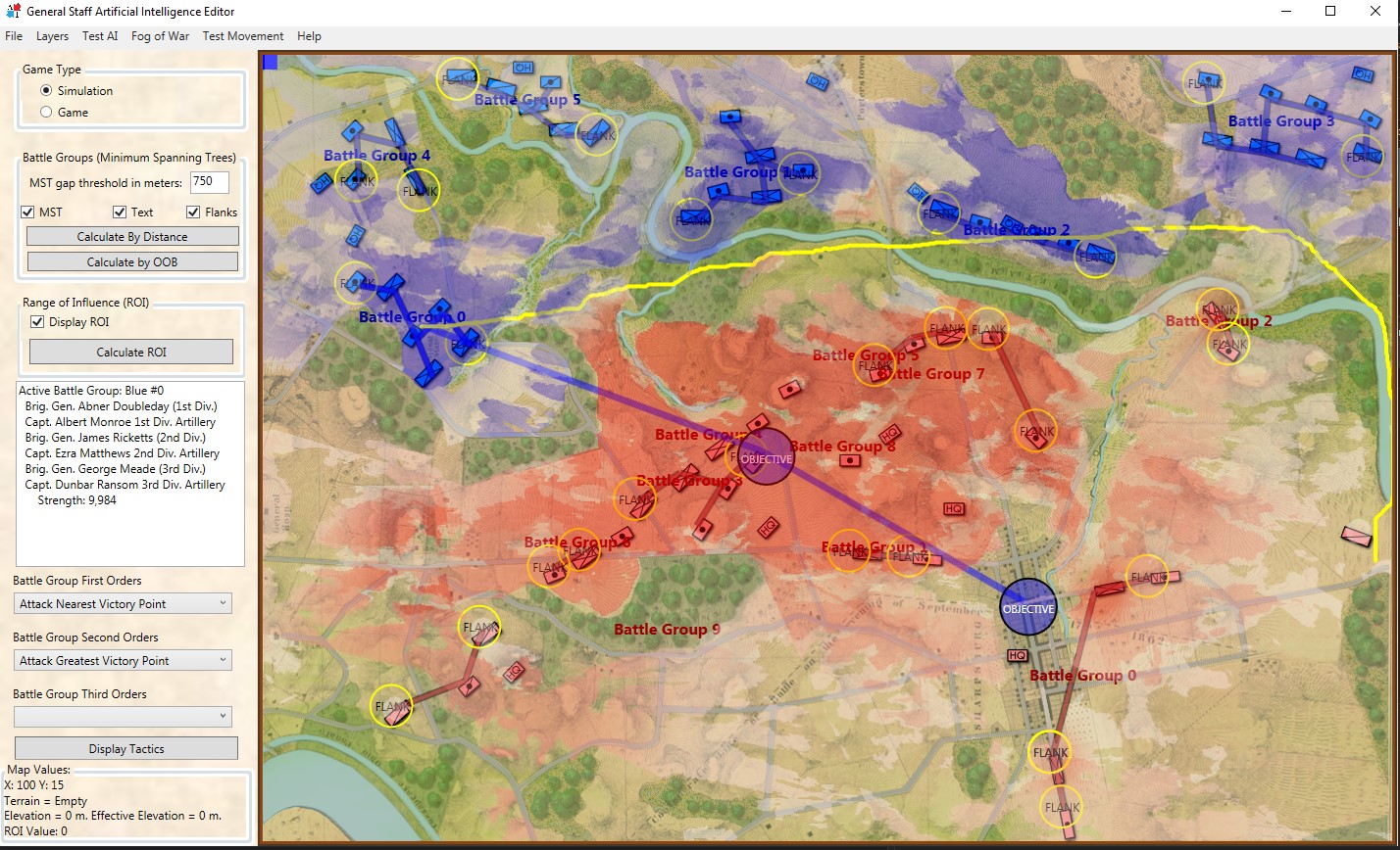
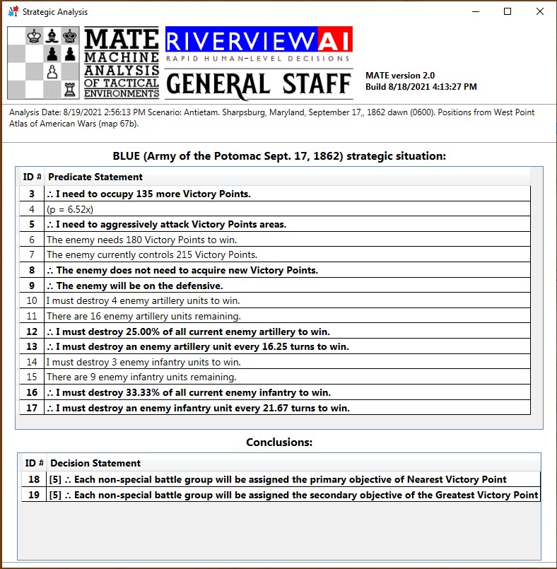
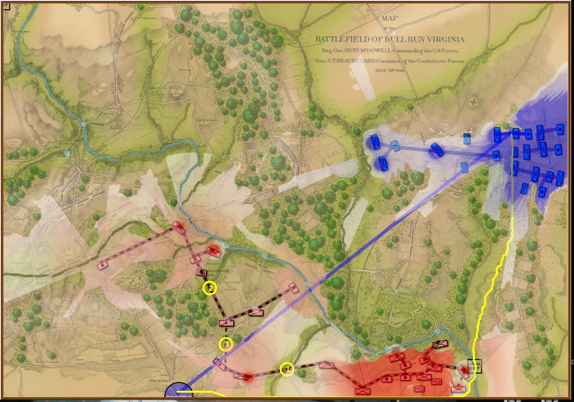
Below is MATE’s analysis from the Blue (L’Armée du Nord) perspective. MATE correctly identifies the key positions and realities of the battlefield:
- Red is on the defensive
- Red has an exposed flank
- There are two key choke points on the route to Red’s exposed flank
MATE then creates an appropriate Course of Action (COA) for Blue:
- Battle Group #1 (The French III Corps) is assigned the flanking maneuver.
- Battle Group #0 (The Imperial Guard) is assigned the objective of St. Amand with the support of Battle Group #4 (IV Corps cavalry and reserve artillery).
- Battle Group #2 (IV Corps) demonstrates against Ligny.
- Battle Group #3 (The Cavalry Reserve) seizes Balatre and a crucial bridge located there.
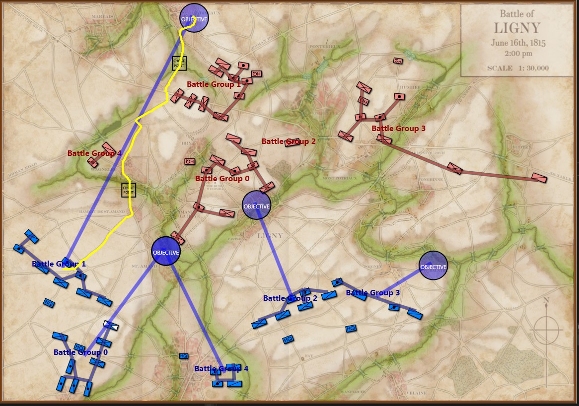
MATE’s analysis of Blue’s position at Ligny. Screen capture. Click to enlarge.
A log of MATE’s thought processes, with my commentary, follows:
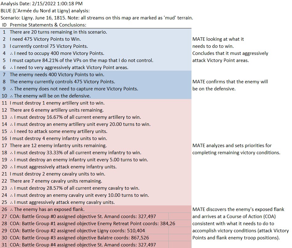
Text output of MATE’s analysis of Blue’s position at Ligny. Click to enlarge.
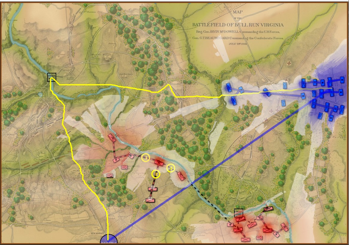
MATE also analyzed Ligny from the Prussian (Red) perspective:
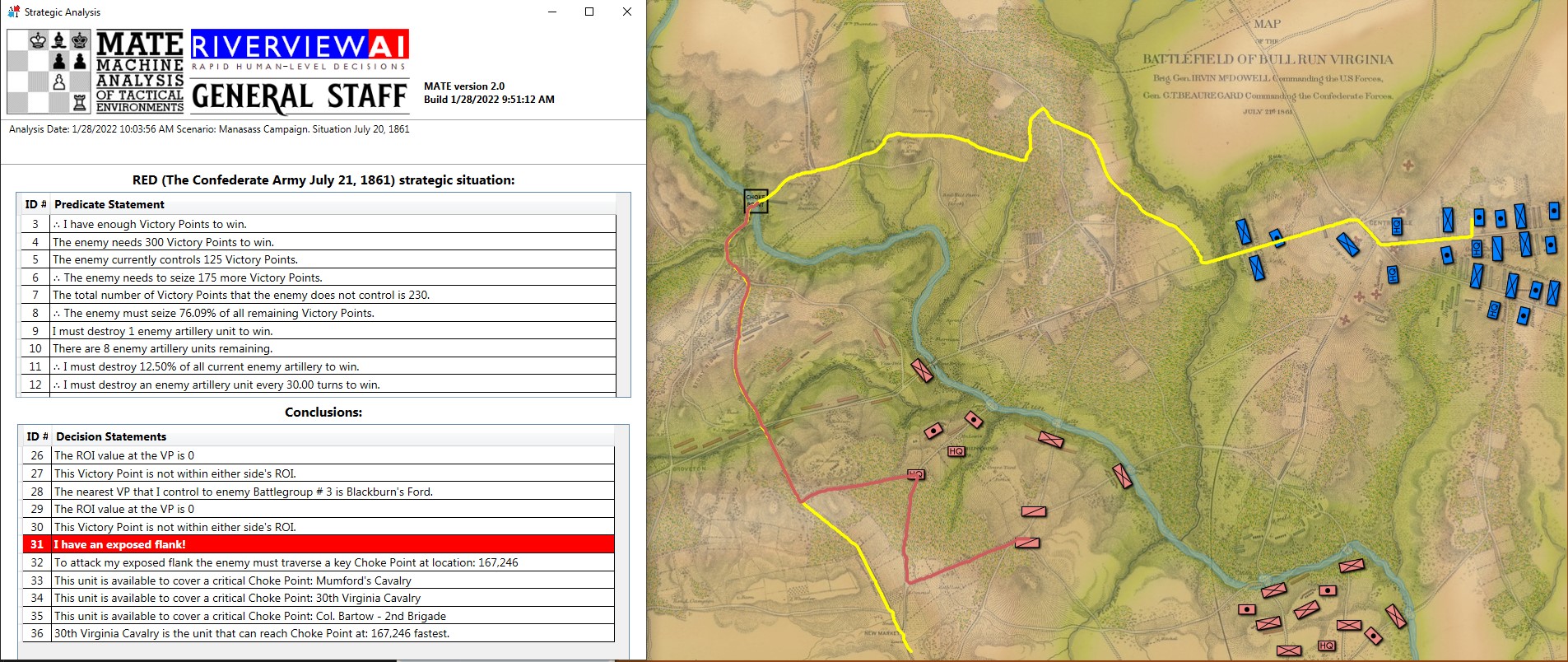
Screen capture of MATE’s analysis of Ligny for Red (Prussian army). MATE recognizes the two choke points on the route of the enemy’s flank attack and dispatches cavalry units to cover these critical areas. Click to enlarge.
MATE, analyzing the Prussian (Red) position correctly recognizes that it is on the defensive, it has an exposed flank, there are two crucial choke points on the route that Blue will take on its flanking maneuver and dispatches two cavalry units to cover the bridges. A log of MATE’s thought processes, with my commentary, follows:
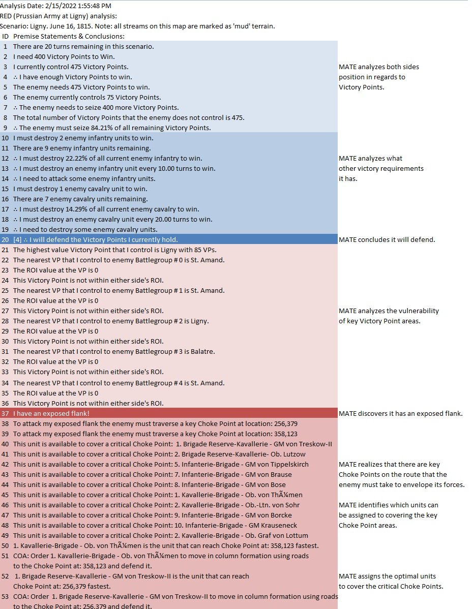
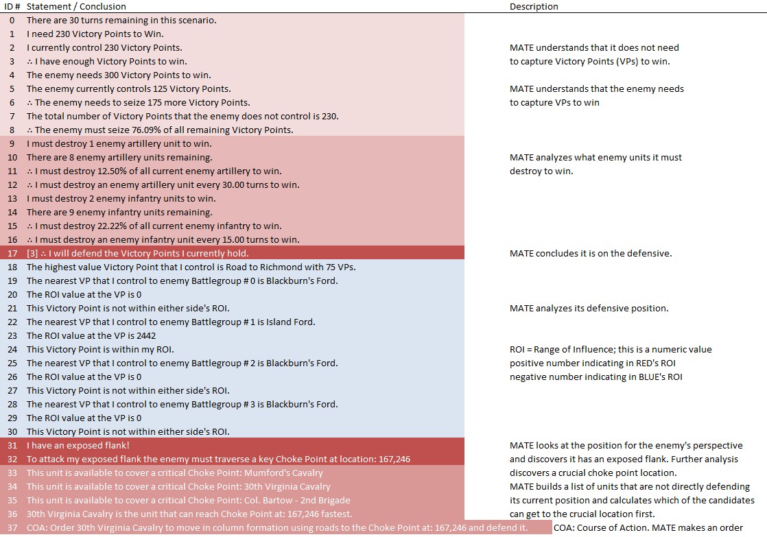
Text output of MATE’s analysis of Red’s position at Ligny. Click to enlarge.
Critique of MATE’s analysis:
As the author of MATE any critique I have of its performance should be taken with a grain of salt (also, see this video). If I was back in academia I would put together twenty or thirty Subject Matter Experts (SMEs), set up a double blind web site, get all the SME’s solutions to the problem, and compare their solutions to MATE’s. If they match to a statistical significance it proves the ‘human-level’ part. But, I’m not in academia anymore and you’ll just have to take my word for it. That said, MATE did what I expected it to do.
It first sussed out if it was on offense or defense and what it had to do to win.
Then, as Blue, MATE discovered a back door to Red’s position and ordered a classic enveloping maneuver. MATE assigned Blue Battle Group #1 the task of implementing the flanking maneuver. Blue Battle Groups #0, #4 and #2 are the fixing force. See my paper, Implementing the Five Canonical Offensive Maneuvers in a CGF Environment (free download here) for details and algorithms. The Blue Cavalry Reserve is given the COA to seize the town of Balatre. This, in my opinion, is a pretty good tactical plan.
When MATE finds itself on defense, as it does as Red at Ligny, one of the first things it does is ask itself, “how would I attack myself?” So, of course it finds the back door right away. Then it compiles a list of available units that are not actively engaged in holding crucial parts of a defensive line, selects the optimal (fastest) units and assigns them orders to defend the crucial choke points. This was a better plan than Field Marshal Gebhard Leberecht von Blücher had. So, again, I’m going to argue that MATE is operating at a ‘human-level’.
As always, please feel free to write me with the questions or comments. MATE is going to take a look at Antietam next.
References
| ↑1 | Machine Analysis of Tactical Environments |
|---|