Why is this wargame taking so long? The short answer is that I made a series of bad decisions. The longer answer involves explaining the bad decisions.
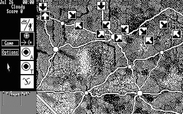
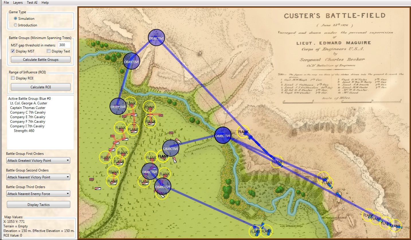
Before I began work on General Staff: Black Powder I had done a project for the US Army called MARS (Military Advanced Real-Time Simulator).
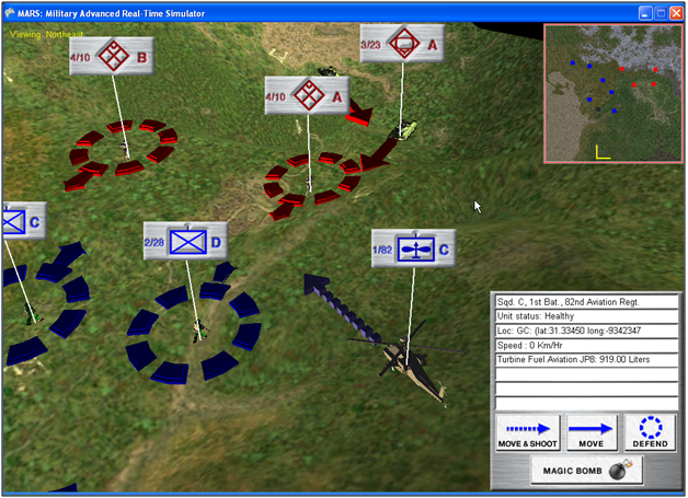
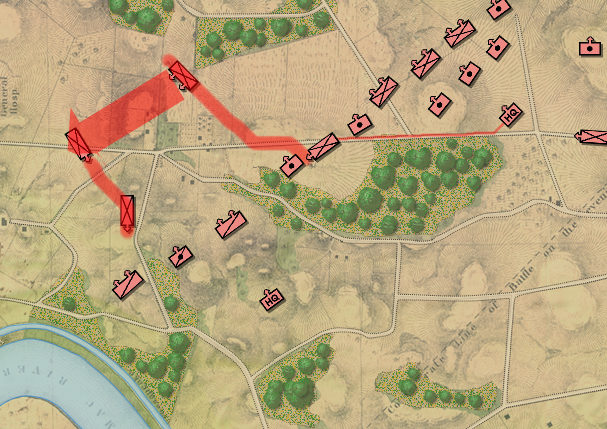
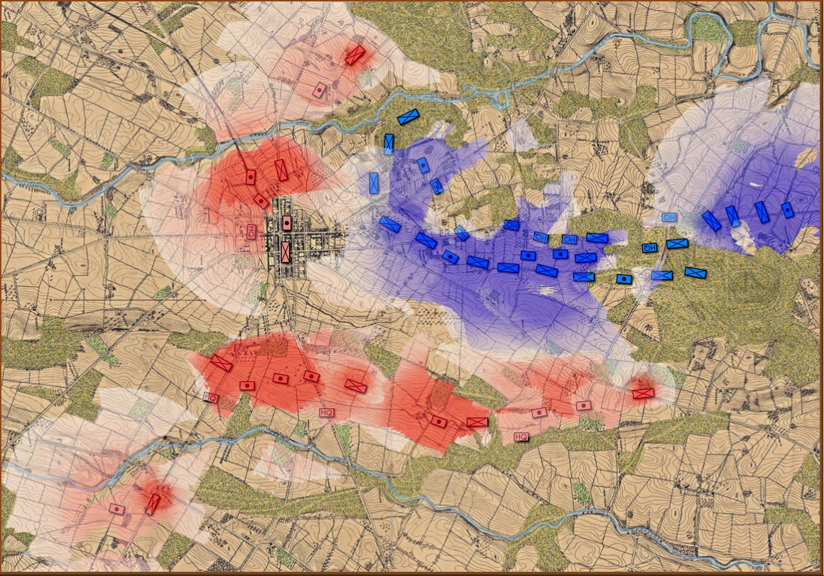
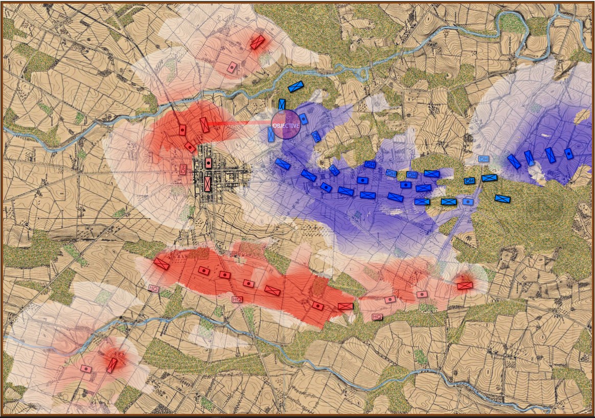
Image from the MARS: Military Advanced Real-Time Simulator feasibility report to the US Army. Screen shot of MARS.
I had used a Microsoft IDE (Integrated Development Environment) called XNA to write MARS in C# and I thought it would be a good environment in which to develop General Staff. XNA, on top of being fairly easy to implement a 3D or 2D game environment, had another interesting advantage: any program created with it was immediately portable to the XBox game console. This dovetailed nicely with my dream of someday bringing wargaming to a larger (and younger) audience.
Consequently, the first version of General Staff – including the Army Editor, Map Editor and Scenario Editor – was written using XNA. I had just begun working on the actual game itself when Microsoft suddenly announced that it was no longer supporting XNA. This, of course, sent shock waves through the XNA game development community.
Since I had already written a great deal of the necessary code in C#, and Windows remained my target audience (Windows makes up >90% of the gaming market) I decided to port (that’s a game development word for rewrite for another environment, but hopefully not rewrite everything) to Microsoft Windows Presentation Foundation (WPF).
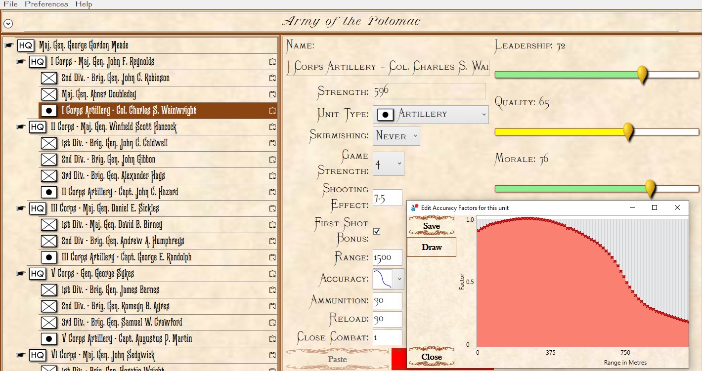
I wasn’t thrilled about porting to WPF. First of all, I wasn’t that familiar with it and, secondly, it wasn’t easy (at least for me) to do a lot of the things that needed to be done. The Army Editor was a pretty easy port, but the Map Editor had some very specific, difficult problems having to do with drawing on the screen. Luckily, I found Andy O’Neill, who is a certified expert on WPF. Andy took over and decided to rewrite my code (properly for WPF) and, eventually, the Army Editor, Map Editor and Scenario Editors were completed. If you are an early backer of General Staff: Black Powder you should have these. They are also available for download on Steam.
By this point the General Staff: Black Powder suite of editors had now been rewritten three times for two different environments, but, it was finally completed and in a stable version. I have been using these programs to create numerous scenarios (some of which are already uploaded to Steam).
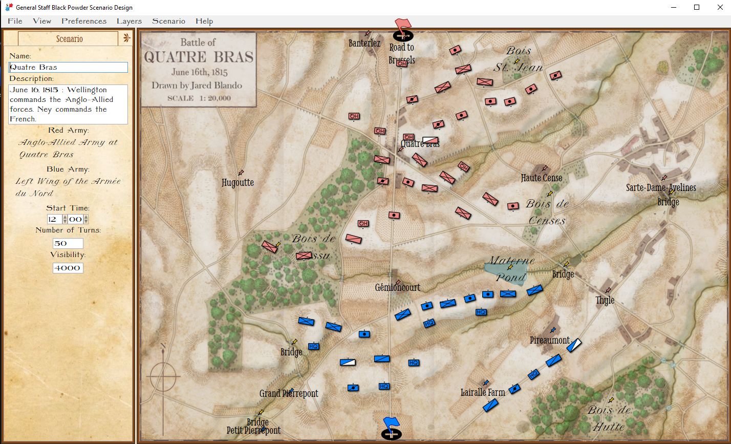
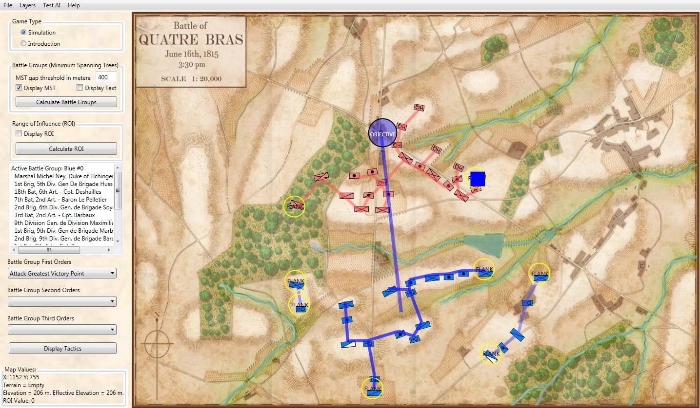
The Quatre Bras scenario in the General Staff: Black Powder Scenario Editor. Screen shot. Click to enlarge.
The last thing to do to complete General Staff: Black Powder was the actual game, or game engine. Usually, this isn’t too hard because about 80% of the code is recycled from the Army, Map and Scenario editors. Unfortunately, I just wasn’t happy with the how the game looked in WPF. WPF is great for creating business apps but it just wasn’t giving me the 19th century Victorian look and feel that I wanted. About this time I discovered that a number of former XNA users had banded together to maintain and expand the original IDE; it was now called MonoGame. I decided to write the General Staff: Black Powder game engine in MonoGame.
I was making pretty good progress, but ran into some problems and asked the MonoGame community for help (by the way, I’ve found the MonoGame community to be a great group for answering newbie questions and generously providing time and solutions). It was on the MonoGame community forum that I met Matthew T. who is an experienced XNA/MonoGame game developer (he has a game on Steam that has sold over 100,000 copies). Matthew, eventually, decided to rewrite large hunks of my MonoGame code (vastly improving it) and then began to add some wonderful debugging features.
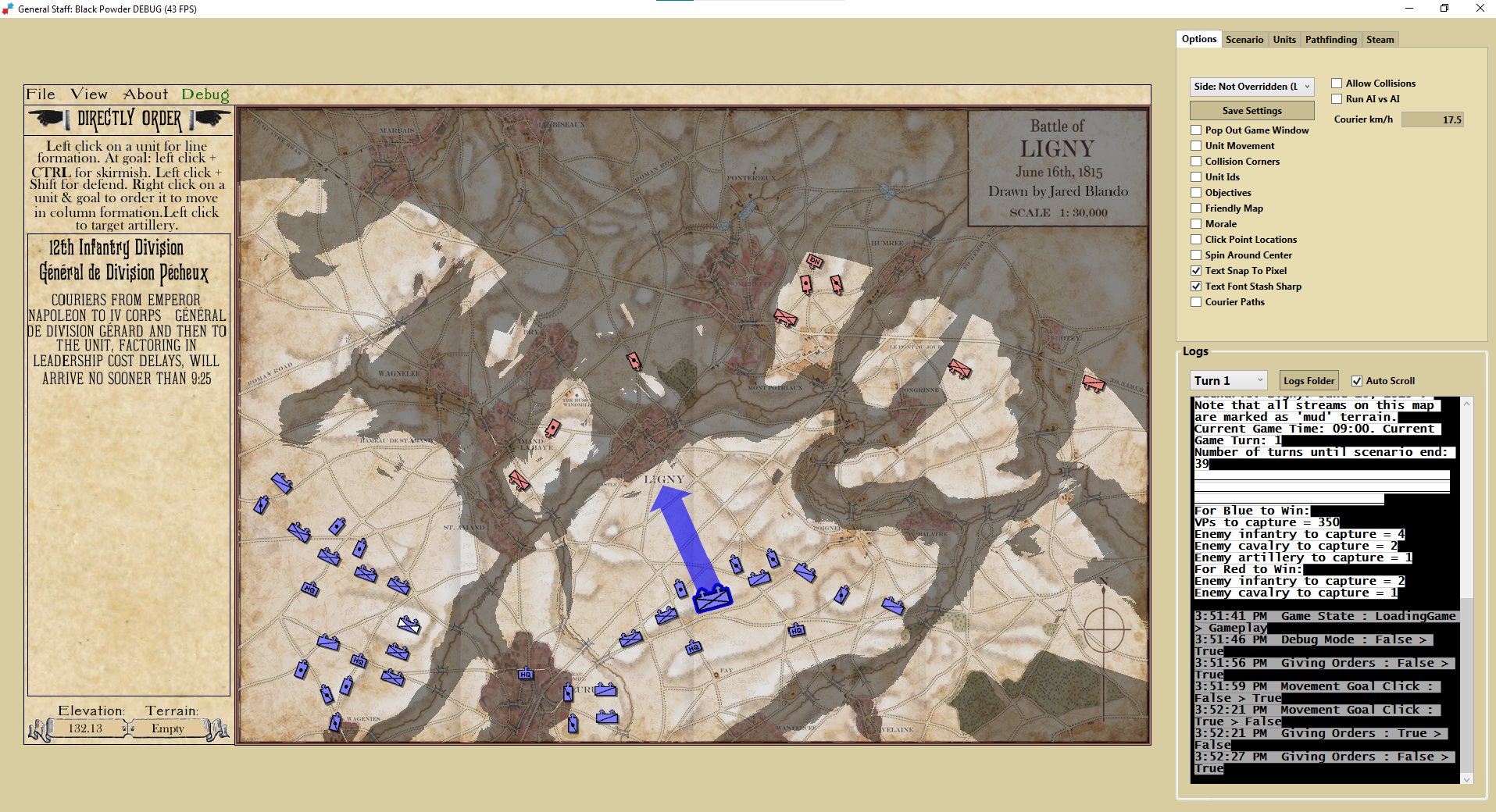
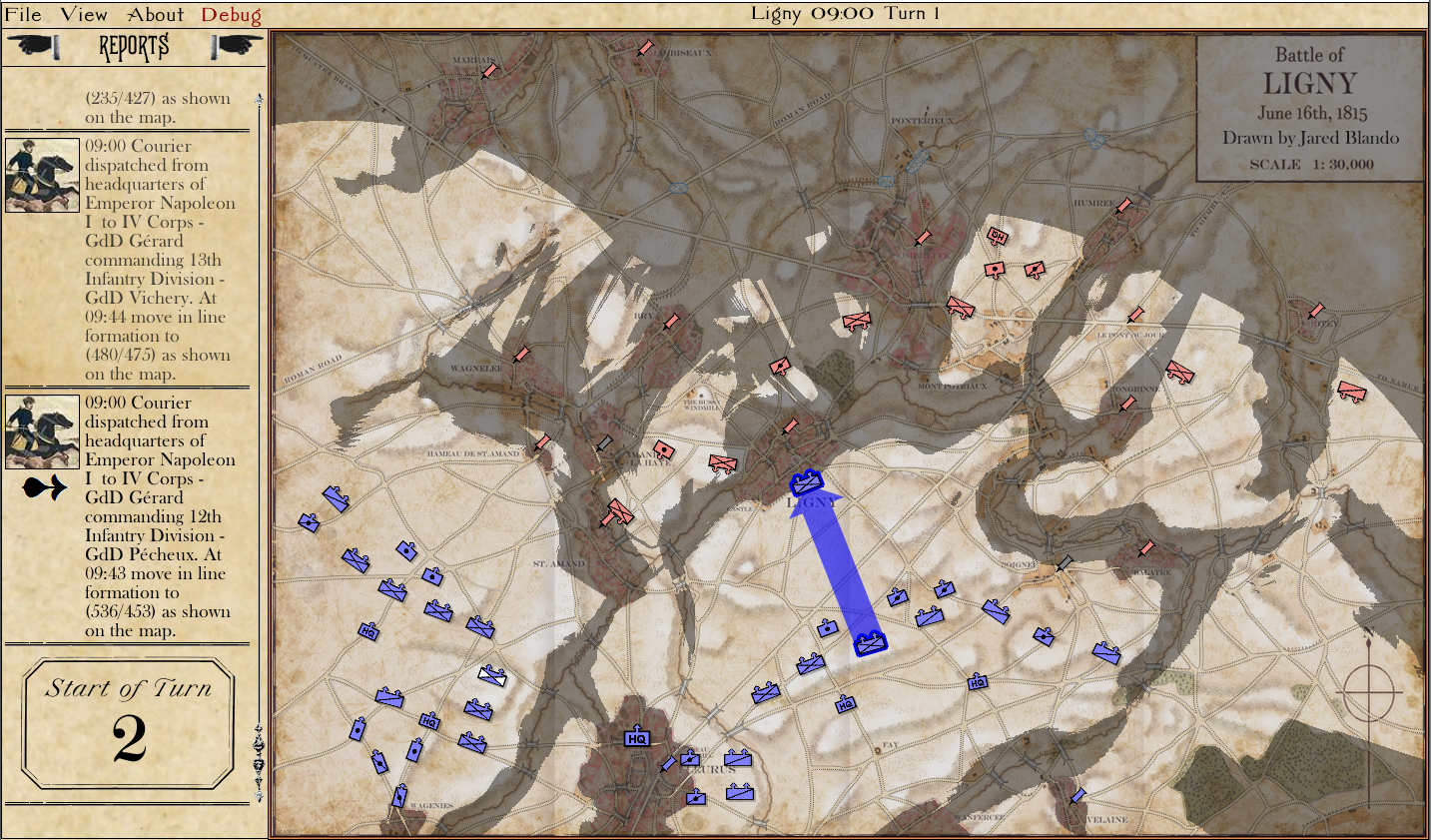
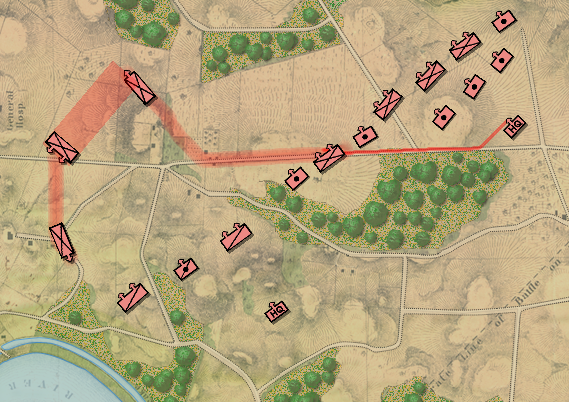
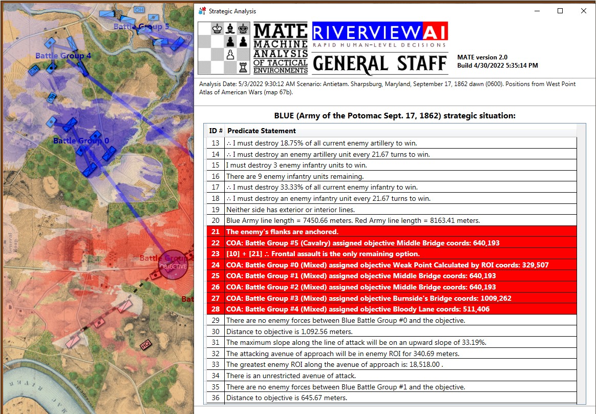
Screen shot of Ligny scenario in General Staff: Black Powder debugger mode. Click to enlarge.
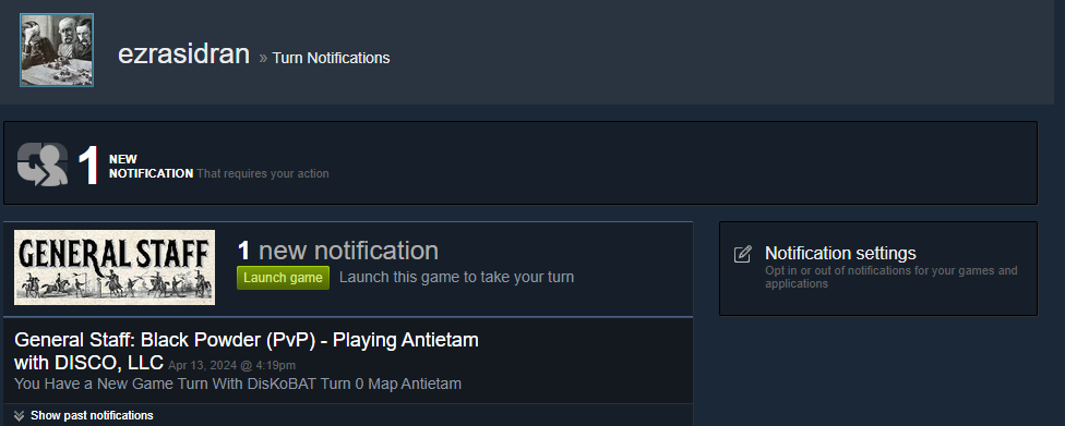
Matthew and Darin Jones also implemented Steam player versus player (PvP) and we’ve done some early playtesting with Matthew in the UK and me in the US playing against each other in real-time (this was an amazing experience and something that I never envisioned that we could pull off).
So, that’s where we are now. We’ve made great progress and we’ve taken far longer to do it than I had hoped or anticipated. A lot of the same code has been written and rewritten for different environments. With 20/20 hindsight I certainly could have managed this a lot better. I think we’re about two months away from a pre-release beta starting with PvP playtesting. This would involve all the early backers who would get new Steam keys.
As always, please feel free to contact me directly with any questions or comments